ECE 4160 Fast Robots

Raphael Fortuna

---

Lab reports made by Raphael Fortuna @ rafCodes Hosted on GitHub Pages — Theme by mattgraham

Summary

In this lab, I added mapping functionality to the robot to map the room in the lab by having it gather data while rotating. The time-of-flight (ToF) sensor was used to gather data and angular speed control was used to control the rotation of the robot. The generated maps were processed in Python and a straight-line map was drawn.

Prelab

I reviewed the lecture on transformation matrices and saw that because the locations to map with the robot were offset from the center, the x and y coordinates of the output map from the robot had to be shifted by that offset to be in the correct location.

Along with this, I used the ToF sensor on the left side of the robot, so I had to add a phase shift to the recorded values so that the first value started on the left side of the robot.

Control Task – Angular Speed Control

The goal for using angular speed control was to have the robot continuously move at 25 degrees per second and record 14 sensor readings spaced out by 1 second. This was to be done using a PID controller that acted directly on the raw gyroscope yaw value – reducing the errors that come from integrating the yaw readings to get the current yaw angle the robot was at from start.

During lab 4, the IMU lab, I had found that the accelerometer had a low pass filter enabled on the chip and so I did not need to low pass the gyroscope yaw values. I used the data gathered in lab 5 to set the base PWM value for turning the robot and tweaked it a little to account for the modifications made to the car.

The car had tape added to its wheels to reduce its static coefficient of friction to make it easier for it to start turning and require a smaller initial PWM value. The left PWM was 102 and the right PWM was 112. I set my target to be 25 degrees per second and because I was turning clockwise, my yaw reading was negative and so my error function was setpoint + angle instead of setpoint – angle to account for this. My PID function is below:

Now with the PID, I needed to gather 14 data points using the ToF sensor. I made a loop that would get ToF values every 1 second and constantly fed in the latest value from the gyroscope to the PID. I collected motor data during this time, and once this was done the car was stopped and the ToF, motor, and raw yaw data was sent to the laptop. My loop code is below.

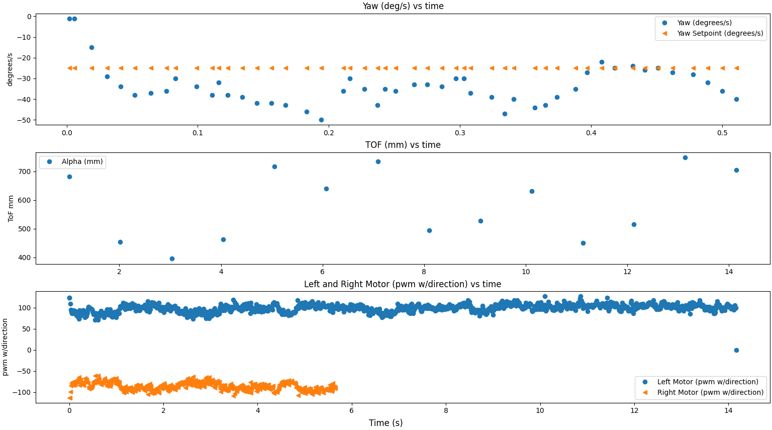
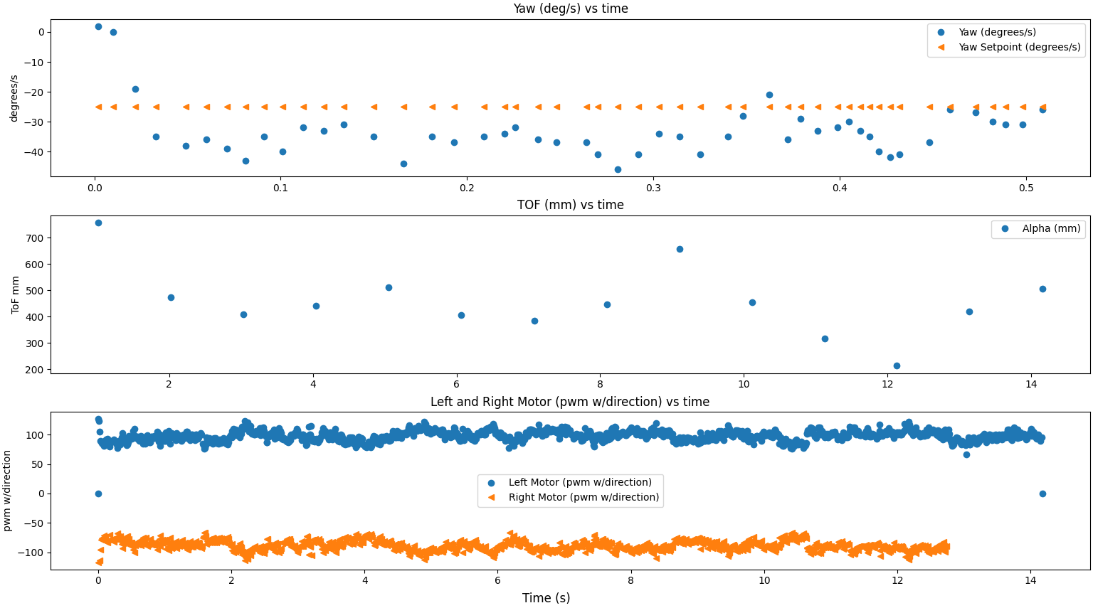
A video of the car mapping at (5, -3) location in the map is shown below. The car started and finished in nearly the same positions and kept itself mostly rotating on its central axis as seen below, with the PID keeping the speed largely in the correct range of degrees as seen below in the graphs. The slowest speed was 20 degrees/s, but the setpoint was 25 degrees/s as per the spec. During the one measurement, the orientation of the robot changed about 25 degrees per second, matching the spec for the angular speed control.

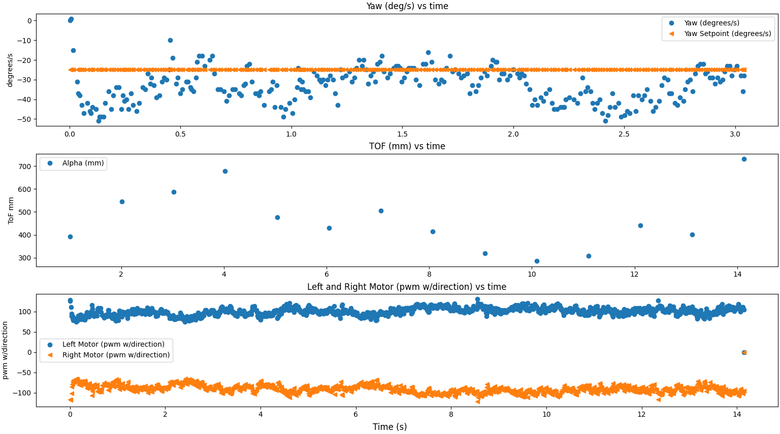
If the robot were spinning in the middle of a 4x4m2 empty, square room, the smallest ToF reading distance would be 2 m and the maximum distance would be 2.82 m. Given that during the mappings for this task the maximum value recorded was .968 m, the robot would struggle to map the room accurately, likely mapping more of a circle of 1 meter than the square it is in. This decrease in range is strange and I will be investigating it further.

Read out Distance Task

Now, I ran the robot in the four locations of the room and took measurements. I started the robot in the same orientation for each of the scans and found that the robot behavior was reliable enough to assume that the readings were equally spaced in angular space by ~25 degrees as it turned at a uniform rate.

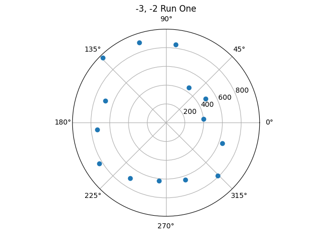
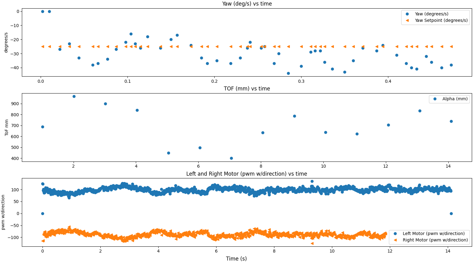
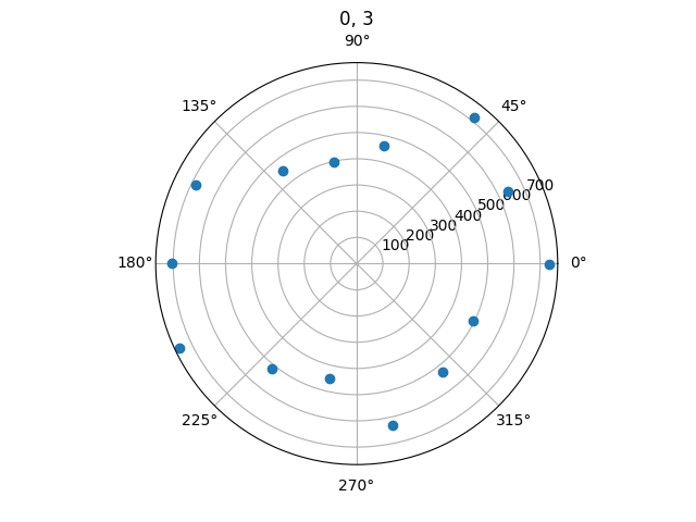
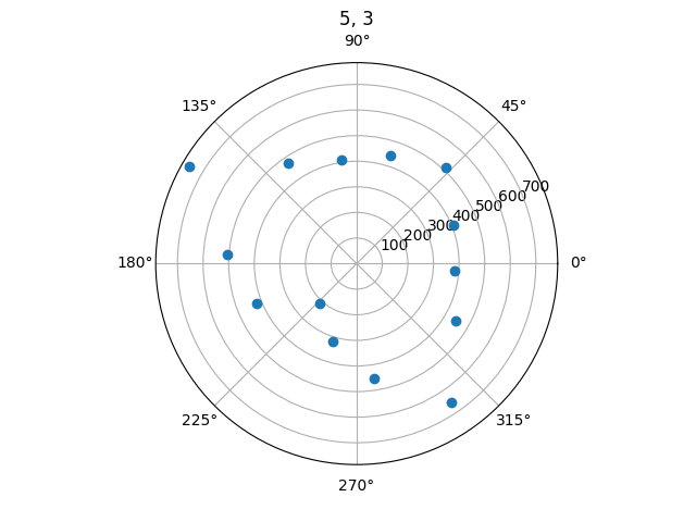
Here are the individual plots plotted in the polar coordinate plot for each point as well as their PID, ToF, motor control graphs.

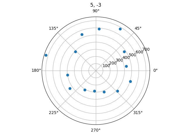
The measurements do not match up exactly with what I expected and is likely due to the maximum range of the sensor of 4m and the sensor returning noisy readings when going past that value.

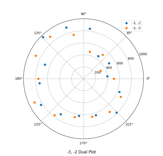
At (-3, -2), I ran the robot two times and found that the graphs roughly matched as can be seen below.

Merge and Plot your Readings Task

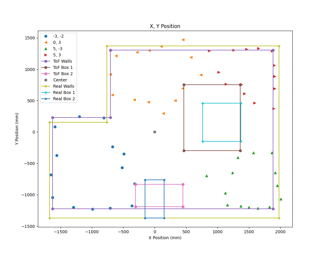
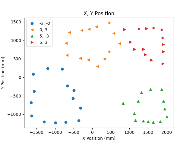
This next task involved assembling the scans into one map. As mentioned before in the Prelab, I added a phase shift to the recorded values (also added above to make it easier to read the data) and found the x and y coordinates of each point by using the cos and sin of the angle where each point multiplied by the radius respectively. Once this was done, I added the x and y shift to each output respectively like [[x], [y]] to transform the coordinates for each measurement set to the inertial reference frame of the room as Anaya discussed on her lab website here. Here are my plotted graphs:

Convert to Line-Based Map Task

I needed to manually estimate the actual walls and obstacles based on the scatter plot. I attached a mouse clicking function to the matplotlib plot so that the x and y coordinates of where I clicked on the graph using the code below:

I saved these as two lists and plotted them on the graph as shown below. There were some corners missing for the two obstacles in the map and I estimated the other corners by some of the detected corners. Here are the lists of the start and end positions of the line segments that make up the walls of the map and the two boxes.

• start box 1 = [(1362, 752), (462, 752), (462, -299), (1362, -299)]
• end box 1= [(462, 752), (462, -299), (1362, -299), (1362, 752)]
• start box 2 = [(-308, -834), (-308, -1189), (451, -1189), (451, -834)]
• end box 2 = [(-308, -1189), (451, -1189), (451, -834), (-308, -834)]
• start wall= [(-706, 1304), (-706, 230), (-1625, 230), (-1625, -1223), (1883, -1223), (1883, 1304)]
• end wall = [(-706, 230), (-1625, 230), (-1625, -1223), (1883, -1223), (1883, 1304), (-706, 1304)]

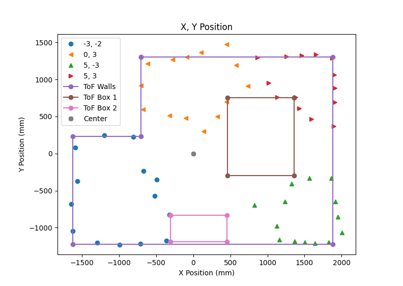
I also went and got the map from Anaya’s website of the real values of the arena last year, which matched this year’s room and found the walls mostly matched, but the obstacles did not match as well. This is likely due to only having 14 measurements and any noise or errors being much more prominent due to the lack of values. The graph of all maps and graphs combined can be seen below. The walls were a little smaller than the actual walls and the obstacles did match on some sides.